Harmonization
Harmonization of DHS and census data
This manual provides a step-by-step guide to harmonizing census and survey data for the purposes of small area estimation (SAE). More specifically, we describe how to create harmonized files of census data from IPUMS International (IPUMSI) and survey data from Demographic and Health Surveys (DHS). These harmonized data files can subsequently be used to construct SAE models for DHS indicator variables.
To motivate the technical instructions in this manual, we consider a case study involving data from the West African nation of Sierra Leone. Our objective is to construct SAE models for three DHS indicators: (1) Any contraceptive use, (2) modern contraceptive use, and (3) unmet need. To do so, we need to assemble harmonized data sets containing all the relevant predictor variables appearing in both the 2015 IPUMS sample and the 2019 DHS sample, as well as the appropriate geographic variables.
The diagram below provides a visual overview of the data harmonization procedure that we introduce in this manual:
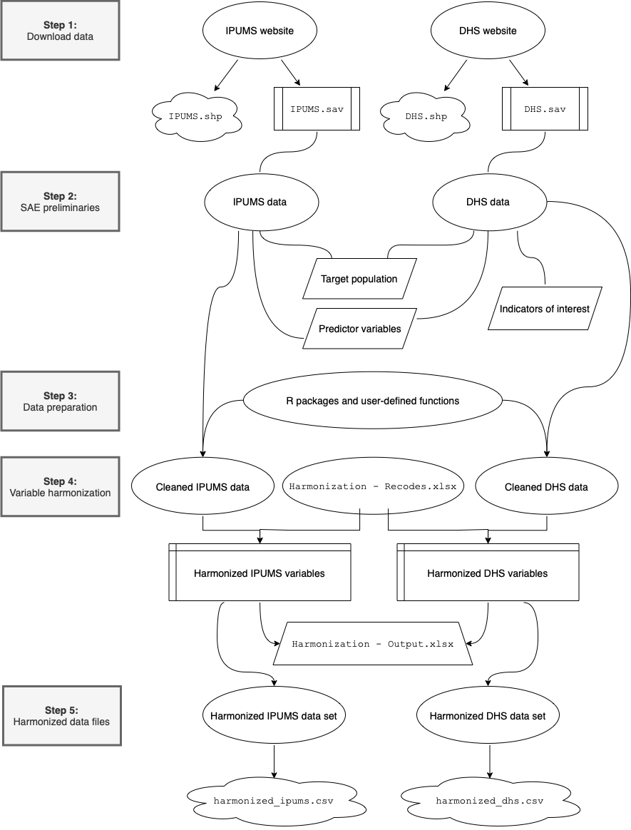
Harmonization flowchart
Step 1: Download data
Step 1A: IPUMS data and shapefiles
Navigate to the IPUMS International homepage (https://international.ipums.org/international):

Harmonization flowchart
If this is your first time downloading data from IPUMS International, you will need to register for an account by clicking the blue “Register” button. If you already have an IPUMS International account, click the “Log In” button in the top right corner of the page.
Once you have logged into your account, you can begin creating a census data extract. Proceed as follows:
- Click on “Select Data”.
- Click the blue “Select Samples” button in the top left corner.
- You should see a column of countries, each with a corresponding row of years for which data are available. Identify the country of interest and check the box to the left of the year for which you would like to download the data. Then click the blue “Submit Sample Selections” button near the top of the page.
- You should now have one sample in your data cart. Next, mark the circular button next to either “Harmonized Variables” or “Source Variables”, depending on which type of variable you would like to use in your analysis. There is no wrong answer here — either harmonized variables or source variables can be used successfully for small area estimation. To read about the differences between the two, see the IPUMS International FAQ page (https://international.ipums.org/international-action/faq). For the Sierra Leone case study, we will use source variables.
- Click the “Display Options” button in the top right corner of the page. Under the “Variable groups” heading, select “Show all groups together”. Then click “Apply Selections”.
- You should now see a long list of variables. Add all of them to your data cart by clicking the circular plus sign next to each variable. Once you have filled your cart with all of the variables, click the blue “View Cart” button in the upper right corner of the page.
- Take a quick look at the list of variables on the next page and verify that everything looks correct. Then click the blue “Create Data Extract” button.
- This will bring you to the extract request page. In the row labeled “Data Format”, click on the word “Change”. Then, under the “Data Format” heading, change the format from “Fixed-width text (.dat)” to “SPSS (.sav)”. Then click the “Apply Selections” button at the bottom of the page.
- If you’d like, you can add a short description of your data extract. Then click “Submit Extract”.
- This will bring you to a page where you can download your extract. Depending on the size of the extract you created, it may take a little while to process. You will receive an email when it is ready to download. To download your data, click the green “Download SPSS” button.
- Give the downloaded file a meaningful name and move it to a suitable directory.
You will also need to download the shapefile for the sample you selected above. For most small area estimation models, the initial model will be constructed at IPUMS’s first administrative level using the survey data, and the model will make predictions at IPUMS’s second administrative level using the census data. In the case of Sierra Leone, for example, the DHS indicators are modeled at the district level (first administrative level), and predictions are made at the chiefdom level (second administrative level).
Navigate to IPUMS International’s GIS boundary files page (https://international.ipums.org/international/gis.shtml). Proceed as follows:
- Click on “Year-specific second-level geography”.
- You should see a list of countries, along with a row of years for which the geographic data are available. Identify your country of interest and click the year for which you downloaded data above.
- This will download a folder containing the corresponding shapefiles. Rename the folder if you’d like, and then move it to the directory from Step 11 above.
Step 1B: DHS data and shapefiles
Navigate to the DHS homepage (https://dhsprogram.com):

Harmonization flowchart
Click on “Login” at the top of the page. If this is your first time downloading DHS data, you will need to register for a new account. If you have downloaded DHS data before, you can log into your existing account.
Once you have logged into your account, proceed as follows to download the survey data and corresponding shapefiles:
- Hover over the “Data” menu at the top of the page and select “Download Datasets”.
- In the blue “Select Country” dropdown menu, select the country of interest.
- You should see a list of surveys from the country of interest. Out of all the Standard DHS samples (see the “Type” column), identify the one closest in year to the IPUMS sample from Step 1A. Ideally, there should be no more than a four- or five-year gap between the IPUMS and DHS samples. In the “Survey Datasets” column, click on “Data Available” for this sample.
- This will bring you to a page containing a long list of data files. Under the “Individual Recode” heading in the “Survey Datasets” section, download the .zip file for the SPSS dataset (.sav). Once this .zip file is downloaded, unzip it. Give the downloaded files meaningful names and place them in the directory from Step 11 above.
- Under the “Geographic Data” heading in the “Geographic Datasets” section, download the .zip file for the shape file (.shp). Once this .zip file is downloaded, unzip it. Give the downloaded files meaningful names and place them in the directory from Step 11 above.
Step 2: SAE preliminaries
Step 2A: Identify DHS indicators of interest
After downloading the data, the first step is to identify which DHS indicator(s) you are interested in modeling. DHS samples contain many variables that record information about a wide range of topics, including health behaviors, family planning, and more. Since the processes of data harmonization and SAE modeling are often motivated by a specific real-world problem, it is likely that you have already identified the indicator(s) of interest.
At this stage, it is helpful to note the name(s) of the DHS variable(s) that can be used to construct these indicator(s). Each variable name is a string of capital letters and numbers, usually beginning with “V”. These variable names can be identified using the Guide to DHS Statistics page (https://dhsprogram.com/Data/Guide-to-DHS-Statistics/index.cfm) on the DHS website:
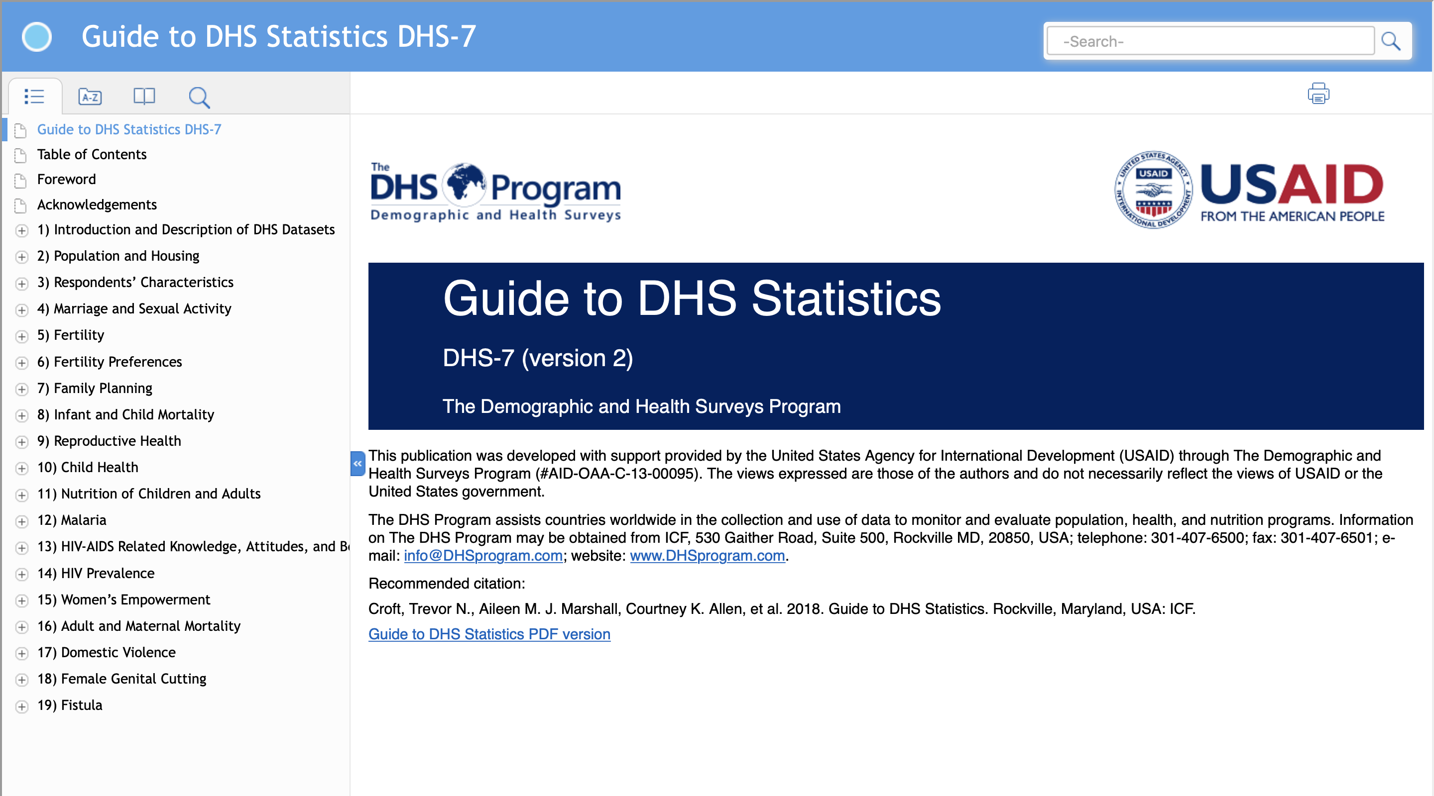
Harmonization flowchart
You can also identify the variable names later, after you load the
DHS data into R in Step 3C.
For the Sierra Leone case study, we are interested in three indicators:
- Any contraceptive use (constructed using V313)
- Modern contraceptive use (constructed using V313)
- Unmet need (constructed using V626)
Step 2B: Identify variables to harmonize
The next step is to identify all the variables that (1) appear in both the IPUMS and DHS samples and (2) could reasonably be used to predict the DHS indicator(s) listed in Step 2A. Here are some common predictor variables that are likely to appear in both the IPUMS and DHS samples:
- Age
- Marital status
- Educational attainment
- Religion
- Number of children ever born
- Number of children surviving
- Urban/rural status
- Employment status
- Occupation
- Literacy
- Primary language
- Ethnicity
- Relationship to household head
- Ownership of durable goods (e.g., car, bicycle, refrigerator, television, radio, phone)
- Household characteristics (e.g., floor material, roof material, wall material, water source, electricity, toilet, cooking fuel)
Note that this list is just a starting point — you may find other variables with predictive potential that appear in both samples.
Just like in Step 2A, it is helpful at this stage to identify the names corresponding to these predictor variables in both the DHS and IPUMS samples. For the DHS data, these variable names can be identified using the Guide to DHS Statistics page (https://dhsprogram.com/Data/Guide-to-DHS-Statistics/index.cfm) on the DHS website — see the screenshot in Step 2A. For the IPUMS data, the variable names can be identified via the variable list for your sample on the IPUMS International website (e.g., https://international.ipums.org/international-action/variables/samples?id=sl2015a):
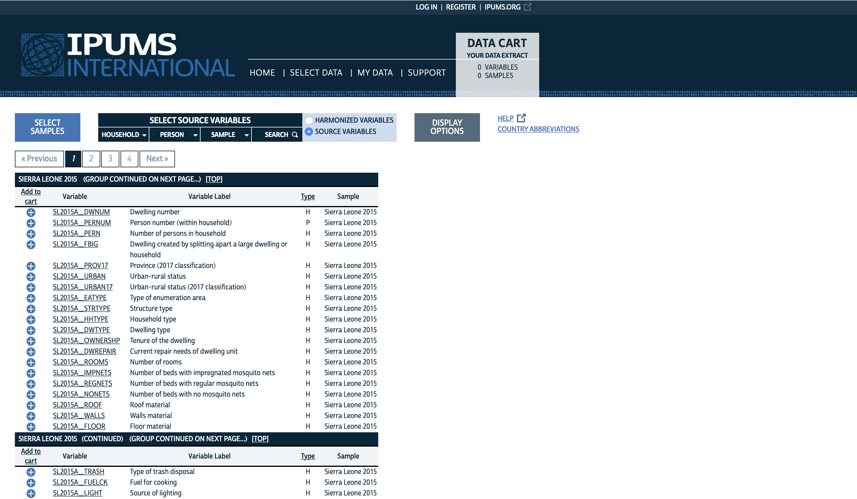
Harmonization flowchart
You can also confirm the variable names for your predictors after you
load the IPUMS and DHS data into R in Steps 3B and 3C,
respectively.
In some cases, one variable in either the IPUMS or DHS sample may be
comparable with a combination of two or more variables in the other
sample. For example, variable V125 from the Sierra Leone
DHS data records whether the individual resides in a household that owns
a car or a truck. However, in the Sierra Leone IPUMS data, this
information is split up into two variables: SL2015A_CAR
records whether the individual lives in a household that owns a car,
while SL2015A_TRUCK records whether the individual lives in
a household that owns a truck.
You will also need to harmonize the survey area variable, which is typically the first IPUMS administrative level. This variable should, by the principles of SAE, appear in both the DHS sample and the IPUMS sample. In the case of Sierra Leone, district is the survey area variable.
I would suggest making a spreadsheet to keep track of the variable names from each sample. Here is a short example for the Sierra Leone data:
At this stage, you should also identify the census area variable, which is typically the second IPUMS administrative level. By the principles of SAE, this variable should appear in the IPUMS sample, but not the DHS sample. Thus, you cannot harmonize the census area across the two samples, but it is worthwhile to identify the variable name associated with it. In the case of Sierra Leone, chiefdom is the census area variable.
Step 2C: Determine target population
You should also determine the target population for your analysis — i.e., the demographic subset that is comparable across the IPUMS and DHS samples. Four characteristics that often (but not always) define the target population are:
- Sex
- Since censuses collect data for respondents of both sexes, this is primarily a concern for the DHS sample. Are the DHS indicators of interest recorded for women only, men only, or both? (Note that if you know this in advance, you can also filter by sex when downloading the DHS data in Step 1B.)
- Age
- Since censuses collect data for respondents of all ages, this is primarily a concern for the DHS sample. DHS typically collects data only for individuals aged 15-49 (or 15-59).
- Household ownership
- Were the data in each sample collected from individuals in private households, collective dwellings, or both? This needs to be confirmed for both the IPUMS and DHS samples. DHS typically collects data only from private households, but censuses may collect data from collectives for some variables. This information can be retrieved from census documentation, which is often available on either the IPUMS website or the national statistical office of the country of interest. It can also be useful to check the universe tab (e.g., https://international.ipums.org/international-action/variables/SL2015A_0404#universe_section) for individual variables in the IPUMS sample.
- Residence status
- Were the samples extracted from a de jure population or a de facto population? In a de jure survey/census, each respondent is enumerated based on their usual residence, regardless of where they are located on the day of the survey/census. In a de facto census, each respondent is enumerated based on their location on the day of the survey/census, regardless of where they usually reside. De jure/de facto status can usually be retrieved from census and DHS documentation.
In some cases, other variables (e.g., marital status, household occupancy/vacancy) may also shape the target population. It is important to consider the unique circumstances of your research question and analysis plan. For the Sierra Leone case study, the target population is the de facto population of women aged 15-49 in occupied, private households.
Step 3: Data preparation
For the remainder of this manual, we will illustrate the processes of data cleaning and harmonization using data from Sierra Leone. Please note that while the general procedures in Steps 3, 4, and 5 are applicable to other SAE projects, the specific tasks required for other projects may vary.
If you do not already have R and RStudio
downloaded on your computer, you will need to download them before
proceeding. This page (https://cran.r-project.org) provides instructions for
downloading R, and this page (https://www.rstudio.com/products/rstudio/download/)
provides instructions for downloading RStudio. Once you
have downloaded them, create a new R script called
[Country name] harmonization.R.
Step 3A: Packages and user-defined functions
Before reading in the data sets you downloaded in Step 1, load the
following packages into R using the library()
function.
library(foreign)
library(tibble)
library(haven)
library(expss)
library(dplyr)
library(openxlsx)
Note: If you have not previously one or more of these packages, you
will need to install them using the install.packages()
function (e.g.,
install.packages(“foreign”)).
We will also make use of four user-defined functions that are
designed to clean up the harmonization process:
compare_categories(), new_var_label(),
write_ipums_output(), and write_dhs_output().
See the Appendix to read about these functions in detail. Feel free to
ignore these details for now, though — you can always refer back to them
later.
Step 3B: IPUMS data preparation
First, identify the path to the IPUMS data file you downloaded in Step 1A:
path_ipums = "~/_OriginalData/SierraLeoneIPUMS2015/sl2015a_ipums.sav"Next, store the IPUMS data file as a data frame. It may be helpful to store an original version of the data frame and make a copy for your actual analysis:
# Store original
sl2015_ipums_orig = read.spss(path_ipums, to.data.frame = TRUE)

# Make copy
sl2015_ipums = sl2015_ipums_orig
If you’d like, you can use the View() and
colnames() functions to view a list of the names of all of
the variables in the IPUMS data frame. This may be helpful if you did
not identify the names of all of your predictor variables in Step
2B.
View(colnames(sl2015_ipums))For the Sierra Leone data, it is necessary to convert age to a numeric variable, as it was categorical by default. This is an example of a country-specific data cleaning task. You may not need to do this for other countries, but you may also find that adjustments need to be made for other variables.
levels(sl2015_ipums$SL2015A_AGE)[1:3] = c("0", "1", "2")

levels(sl2015_ipums$SL2015A_AGE)[which(levels(sl2015_ipums$SL2015A_AGE) == "101+ years")] = "101"

sl2015_ipums$SL2015A_AGE = as.numeric(sl2015_ipums$SL2015A_AGE) - 1
Finally, filter the data frame to obtain the target population identified in Step 2C. You may need to explore the data frame a bit to figure out how to do this.
sl2015_ipums = sl2015_ipums[(sl2015_ipums$SL2015A_SEX == "Female" &
                               sl2015_ipums$SL2015A_AGE >= 15 & sl2015_ipums$SL2015A_AGE <= 49 &
                               sl2015_ipums$SL2015A_HHTYPE == "Household"),]
Step 3C: DHS data preparation
Here, we essentially reapply the procedures from Step 3B for the DHS sample. First, identify the path to the DHS data file you downloaded in Step 1B:
path_dhs = "~/_OriginalData/SierraLeoneDHS2019/SL_2019_DHS_10012021_1417_61748/SLIR7ASV/SLIR7AFL.SAV"Next, store the DHS data file as a data frame. Again, it may be helpful to store an original version of the data frame and make a copy for your actual analysis:
# Store original
sl2019_dhs_ir_orig = read.spss(path_dhs, to.data.frame = TRUE)

# Make copy
sl2019_dhs_ir = sl2019_dhs_ir_orig
If you’d like, you can use the View() and
attr() functions to view a list of the names of all of the
variables in the DHS data frame. This may be helpful if you did not
identify the names of your indicator(s) of interest in Step 2A or your
DHS predictors in Step 2B.
View(attr(sl2019_dhs_ir, "variable.labels"))At this point, you may need to clean the data and/or filter it in some way to obtain the target population, much like we did in Step 3B. For the DHS data from Sierra Leone, neither of these tasks were necessary.
Next, you will need to rescale the individual sample weight variable
(V005) by dividing it by 1,000,000. Then use the
user-defined function new_var_label() to assign a label to
the new weight variable. This new variable label should be the original
label concatenated with “(recode)”.
# Rescale sample weight
sl2019_dhs_ir$V005R = sl2019_dhs_ir$V005/1000000

# Add variable label
sl2019_dhs_ir = new_var_label(sl2019_dhs_ir,
                              "Women's individual sample weight (6 decimals) (recode)")
Step 3D: Create supporting files
The final step before beginning the harmonization process is to create some supporting documents that will help you along the way.
First, in Excel, create a blank workbook called
[Country name] Harmonization - Output.xlsx. You will send
weighted frequency tables of the harmonized variables to this workbook
in Step 4. Also, in R, use the
createWorkbook() function to create an empty object that
will help you send the harmonized output to Excel.
sl_harmonization_output = createWorkbook()Next, in Excel, create a blank workbook called
[Country name] Harmonization - Recodes.xlsx. You will use
this to stay organized during the process of category harmonization.
Each sheet of this workbook should look something like the
following:
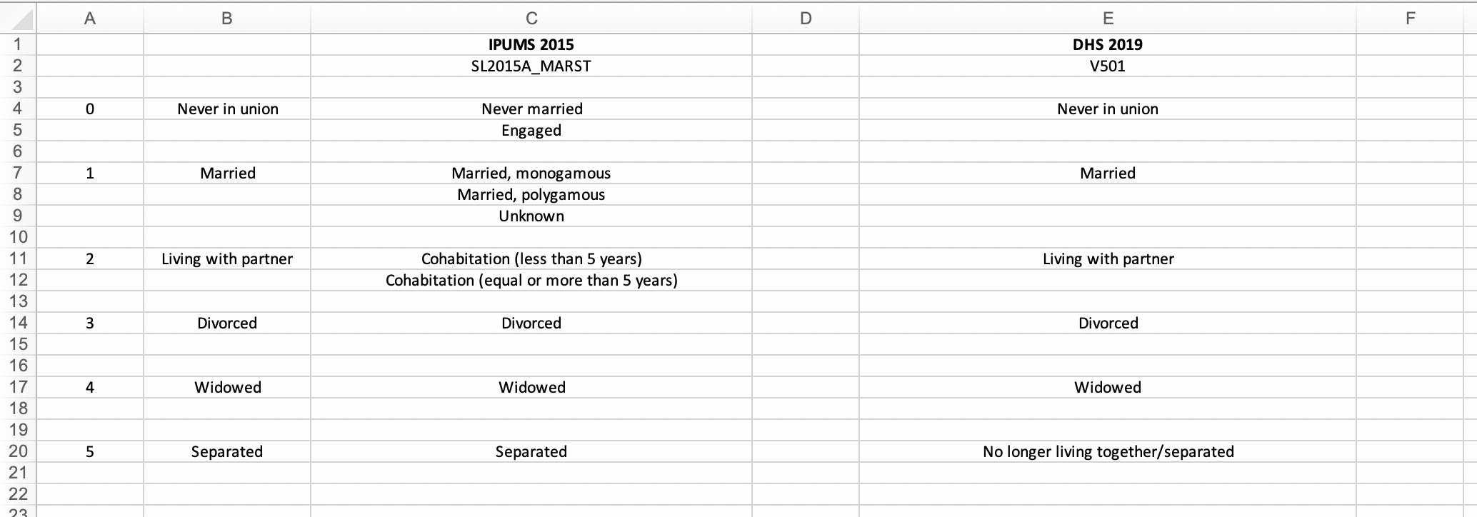
Harmonization flowchart
Finally, create a document to take notes, either in Microsoft Word, Google Docs, or your preferred note-taking software. Aligning the categories of different variables between the IPUMS and DHS samples requires some decision making, so you will want a space to jot down your justifications for these decisions.
Step 4: Variable harmonization
Step 4A: Category alignment
The easiest way to demonstrate the harmonization process is through
specific examples, so we will describe the harmonization of the
religion variable for the Sierra Leone data. It is
reasonable to assume that a woman’s religion might influence her use of
and/or demand for contraception, so we would like to include
religion in our models for the three DHS indicators.
In Step 2B, we identified V130 as the religion variable
from the DHS sample and SL2015A_RELIG as the religion
variable from the IPUMS sample. First, as an exploratory task, we use
the user-defined function
compare_categories()' to run a quick weighted tabulation on these two variables. Note that we use the individual sample weightsV005RandPERWT`
to weight the DHS and IPUMS samples, respectively.
compare_categories(ipums_data = "sl2015_ipums", ipums_var = "SL2015A_RELIG",
                   ipums_weight = "PERWT", dhs_data = "sl2019_dhs_ir",
                   dhs_var = "V130", dhs_weight = "V005R")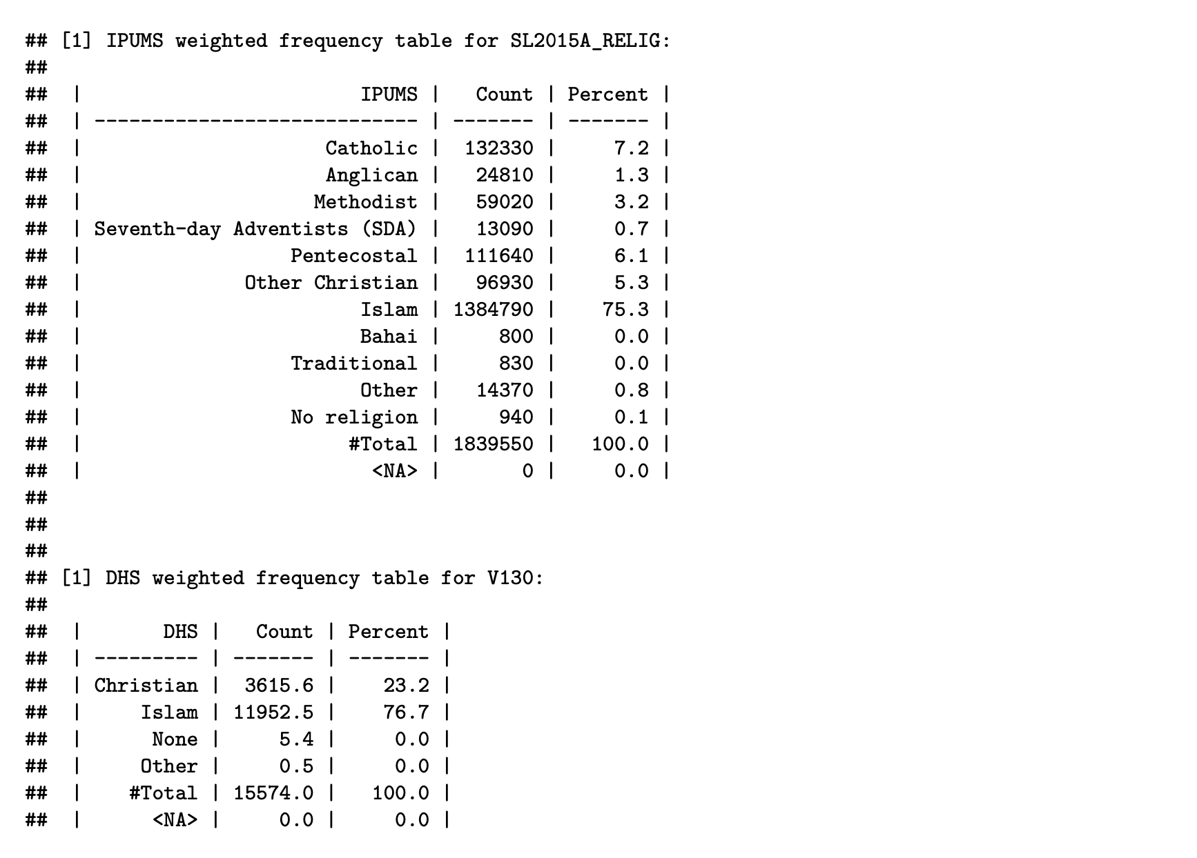
Harmonization flowchart
We find that SL2015A_RELIG has more categories than
V130, so the main harmonization task in this particular
instance will be to consolidate the categories of
SL2015A_RELIG to match those of V130.
I suggest moving out of RStudio temporarily and aligning
these categories in the Excel workbook
[Country name] Harmonization - Recodes.xlsx from Step 3D.
The finished product can be seen below:
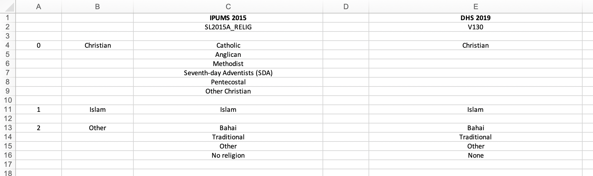
Harmonization flowchart
A couple things to note:
- Column C contains the categories from the IPUMS variable
SL2015A_RELIG. - Column E contains the categories from the DHS variable
V130. Bahai and Traditional actually are categories of the DHS variableV130, but they do not show up in the weighted frequency table above because zero cases were recorded in each of them. - Column B contains the harmonized variable labels, which were determined during this process of category alignment. Column A contains an arbitrary numbering of these harmonized variable labels.
Harmonizing SL2015A_RELIG and V130 is
relatively straightforward. The six Christian denominations in
SL2015A_RELIG can be matched with the single Christian
category in V130. In both variables, there is one category
for Islam, so these can be aligned next. In the weighted frequency
tables above, we observe that Christianity and Islam account for close
to 100% of the cases in both variables, and none of the remaining
categories in either SL2015A_RELIG or V130
have a significant number of cases. Therefore, it makes the most sense
to combine the remaining labels into a harmonized category called
“Other”.
Step 4B: Create harmonized IPUMS and DHS variables
Now we will move back into RStudio and create the
harmonized variables for both IPUMS and DHS. First, use the
fre() function from the expss package to save
a copy of the weighted frequency table from above:
freq_RELIG = fre(sl2015_ipums$SL2015A_RELIG, weight = sl2015_ipums$PERWT)Next, use the factor() and ifelse()
functions to create the harmonized IPUMS variable. If you are unfamiliar
with these functions, you can check out their respective help pages here
(https://www.rdocumentation.org/packages/base/versions/3.6.2/topics/factor)
and here (https://www.rdocumentation.org/packages/base/versions/3.6.2/topics/ifelse).
We suggest naming the new variable SL2015A_RELIGR, which is
just the original variable name with the letter “R” appended (“R” stands
for “recode”).
sl2015_ipums$SL2015A_RELIGR =
  factor(ifelse(sl2015_ipums$SL2015A_RELIG == "Catholic" |
                 sl2015_ipums$SL2015A_RELIG == "Anglican" |
                 sl2015_ipums$SL2015A_RELIG == "Methodist" |
                 sl2015_ipums$SL2015A_RELIG == "Seventh-day Adventists (SDA)" |
                 sl2015_ipums$SL2015A_RELIG == "Pentecostal" |
                 sl2015_ipums$SL2015A_RELIG == "Other Christian",
               "Christian",
               ifelse(sl2015_ipums$SL2015A_RELIG == "Islam",
                      "Islam",
                      ifelse(sl2015_ipums$SL2015A_RELIG == "Bahai" |
                               sl2015_ipums$SL2015A_RELIG == "Traditional" |
                               sl2015_ipums$SL2015A_RELIG == "Other" |
                               sl2015_ipums$SL2015A_RELIG == "No religion",
                             "Other", NA))),
        levels = c("Christian", "Islam", "Other"))
The general idea behind these lines of code is as follows: If an
individual is labeled as “Catholic”, “Anglican”, “Methodist”,
“Seventh-day Adventists (SDA)”, “Pentecostal”, and “Other Christian” in
the original variable, assign them to a category called “Christian” in
the harmonized variable. If they are in the “Islam” category in the
original variable, assign them to a category called “Christian” in the
harmonized variable. If they are assigned to “Bahai”, “Traditional”,
“Other”, or “No religion” in the original variable, assign them to
“Other” in the harmonized variable. If any individuals are not covered
by these three rules, mark them as missing (NA). (Note that
no cases should be missing in the harmonized variable — if you notice
any NA cases when tabulating the harmonized variable, you
should go back and fix this issue.)
Next, use the user-defined function new_var_label() to
assign a variable label to SL2015A_RELIGR. We suggest using
a standard convention variable label where you simply append “(recode)”
to the original variable label:
sl2015_ipums = new_var_label(sl2015_ipums, "Religion (recode)")Finally, check your work by generating a weighted frequency table of the harmonized IPUMS variable:
freq_RELIGR = fre(sl2015_ipums$SL2015A_RELIGR, weight = sl2015_ipums$PERWT)
print(freq_RELIGR[,c(1:2, 4)])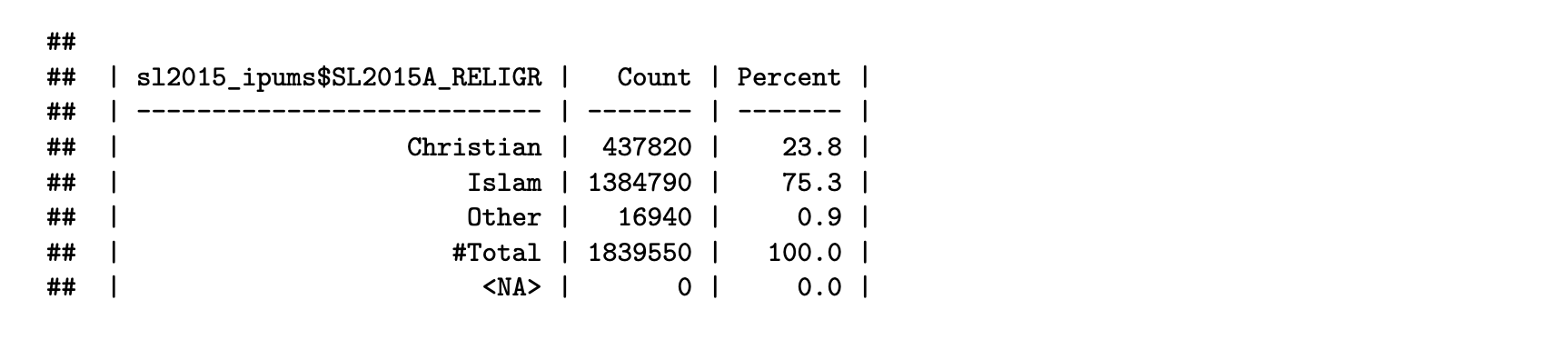
Harmonization flowchart
We have successfully created the harmonized IPUMS variable for
religion, and we can basically apply the same procedures to
create the harmonized DHS variable. First, we save a copy of the
weighted frequency table:
V130_freq = fre(sl2019_dhs_ir$V130, weight = sl2019_dhs_ir$V005R, drop_unused_labels = FALSE)Next, we use factor() and ifelse() to
create the harmonized variable, which we name V130R. We
also add a variable label for V130R:
# Create harmonized DHS variable
sl2019_dhs_ir$V130R = factor(ifelse(sl2019_dhs_ir$V130 == "Christian",
                                    "Christian",
                                    ifelse(sl2019_dhs_ir$V130 == "Islam",
                                           "Islam",
                                           ifelse(sl2019_dhs_ir$V130 == "Bahai" |
                                                    sl2019_dhs_ir$V130 == "Traditional" |
                                                    sl2019_dhs_ir$V130 == "Other" |
                                                    sl2019_dhs_ir$V130 == "None",
                                                  "Other", NA))),
                             levels = c("Christian", "Islam", "Other"))

# Add variable label
sl2019_dhs_ir = new_var_label(sl2019_dhs_ir, "Religion (recode)")
Finally, we generate a weighted frequency table for the harmonized DHS variable:
V130R_freq = frequency(sl2019_dhs_ir$V130R, weight = sl2019_dhs_ir$V005R, drop_unused_labels = FALSE)
print(V130R_freq[,c(1:2, 4)])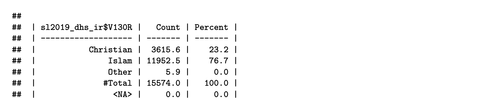
Harmonization flowchart
Step 4C: Write harmonization output to Excel
Now that we have created the harmonized variables for both the IPUMS
data and the DHS data, we can organize our work in the Excel workbook
[Country name] Harmonization - Output.xlsx that you created
in Step 3D. Use the addWorksheet() function from the
openxlsx package to create a new sheet called “Religion”
within your workbook:
addWorksheet(sl_harmonization_output, "Religion")Next, use the user-defined functions
write_ipums_output() and write_dhs_output() to
paste the weighted frequency tables for the harmonized IPUMS and DHS
variables into this Excel sheet:
write_ipums_output(workbook_name = sl_harmonization_output,
                   sheet_name = "Religion",
                   ipums_data = sl2015_ipums,
                   ipums_var_names = c("SL2015A_RELIGR", "SL2015A_RELIG"),
                   ipums_freq_tables = list(freq_RELIGR, freq_RELIG),
                   output_start_row = 1)

write_dhs_output(workbook_name = sl_harmonization_output,
                 sheet_name = "Religion",
                 dhs_data = sl2019_dhs_ir,
                 dhs_var_names = c("V130R", "V130"),
                 dhs_freq_tables = list(V130R_freq, V130_freq),
                 output_start_row = 1)
Finally, use the saveWorkbook() function to save your
Excel file:
saveWorkbook(sl_harmonization_output, file = "Sierra Leone harmonization - Output.xlsx",
             overwrite = TRUE)
After completing these steps, the “Religion” sheet in
[Country name] Harmonization - Output.xlsx will look like
this:
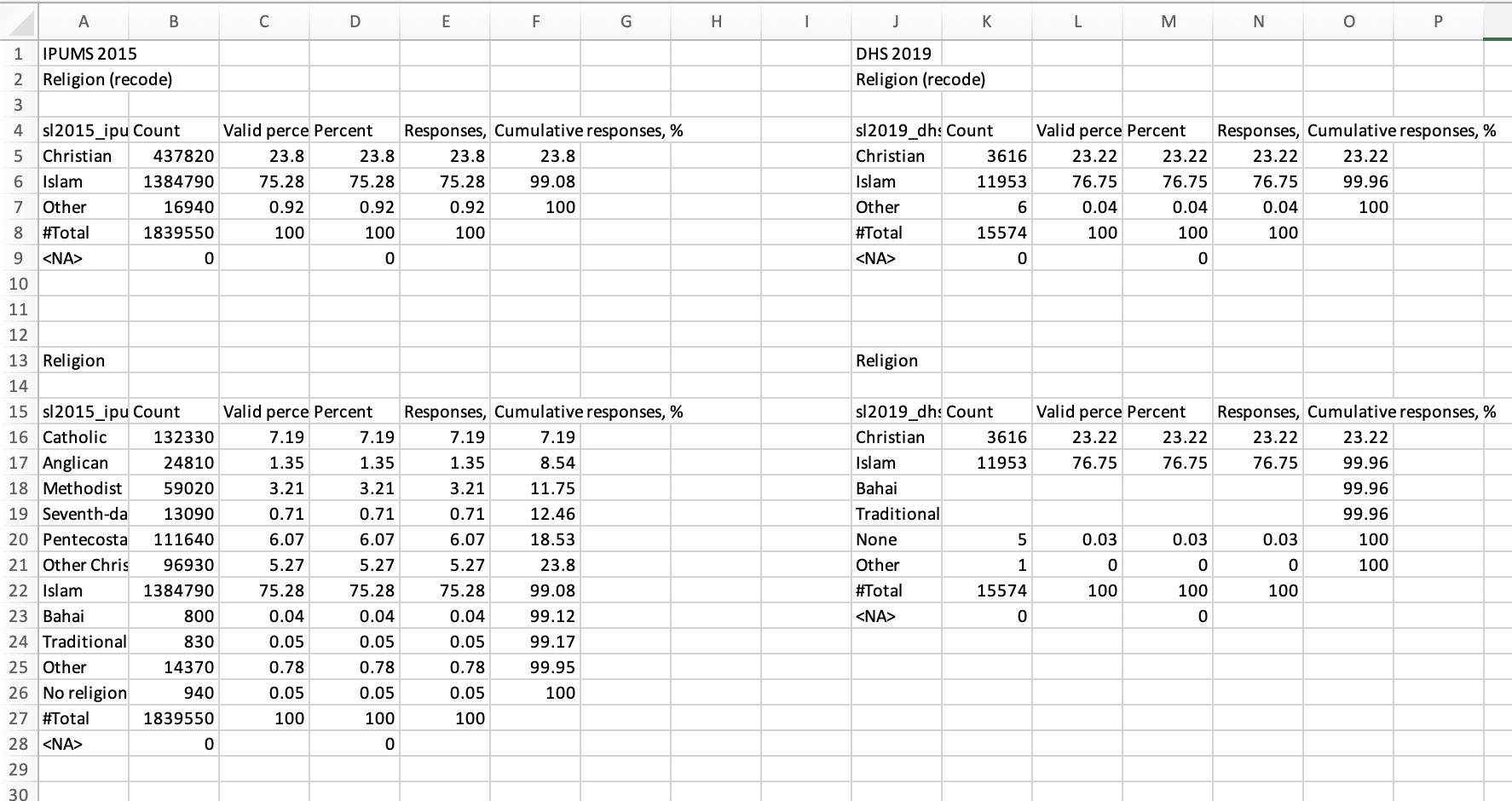
Harmonization flowchart
We can see that the IPUMS variables appear on the left, with the
harmonized variable SL2015A_RELIGR on top and the original
variable SL2015A_RELIG on the bottom. The DHS variables
appear on the right, with the harmonized variable V130R on
top and the original variable V130 on the bottom.
You should compare the percentages in columns C and K for the harmonized variables. Assuming that (1) the DHS data form a representative sample of the IPUMS data and (2) the categories of the variables used to construct the harmonized variables are comparable between IPUMS and DHS, these percentages should be very similar. Here, we see that both of these conditions appear to be satisfied, as the percentages are similar for Christian (23.8% vs. 23.2%), Islam (75.3% vs. 76.8%), and Other (0.9% vs. 0.05%).
Step 4D: Miscellaneous notes
Handling unknown cases:
Some of the variables used to construct the harmonized IPUMS and DHS variables will have cases labeled as “unknown” (or something to that effect). These unknown cases almost always constitute a very small proportion of the total sample, so it typically won’t matter how you classify them in Step 4A. For the Sierra Leone case study, we took the following approach:
- If the harmonized variable has a category called “other” (or something to that effect), simply assign the unknown cases to that category.
- If the harmonized variable does not have a category called “other”, assign the unknown cases to the category with the highest number of cases.
For the religion example above, if there were unknown cases in either
SL2015A_RELIG or V130, we would have assigned
them to the “Other” category in the corresponding harmonized variable.
In contrast, the image in Step 3D illustrates that in the case of
marital status, the unknown cases in the variable
SL2015A_MARST were assigned to the “Married” category
(which must have been identified as the category with the highest number
of cases in SL2015A_MARST).
Creating the DHS indicators:
At this stage, you should also create variables for your DHS indicators of interest (if they are not already in a suitable format in the DHS data set). You can use the same procedures described in Steps 4A through 4C above, although you will not have to worry about the IPUMS-related steps.
For example, we used the following code to create the variable for any contraceptive use, which was one of the three indicators of interest for the Sierra Leone case study:
### Step 4A

compare_categories(ipums_data = NULL, ipums_var = NULL, ipums_weight = NULL,
                   dhs_data = "sl2019_dhs_ir", dhs_var = "V313", dhs_weight = "V005R")


### Step 4B

# Original DHS variable
V313_freq = fre(sl2019_dhs_ir$V313, weight = sl2019_dhs_ir$V005R)

# Harmonized DHS variable
sl2019_dhs_ir$V313R1 = factor(ifelse(sl2019_dhs_ir$V313 == "Folkloric method" |
                                      sl2019_dhs_ir$V313 == "Traditional method" |
                                      sl2019_dhs_ir$V313 == "Modern method",
                                    1,
                                    ifelse(sl2019_dhs_ir$V313 == "No method",
                                           0, NA)),
                             levels = c(1, 0))

# New label for harmonized DHS variable
sl2019_dhs_ir = new_var_label(sl2019_dhs_ir, "Any contraceptive use")

# Weighted frequency table for harmonized DHS variable
V313R1_freq = fre(sl2019_dhs_ir$V313R1, weight = sl2019_dhs_ir$V005R)


### Step 4C

addWorksheet(sl_harmonization_output, "Any contraceptive use")

write_dhs_output(workbook_name = sl_harmonization_output,
                 sheet_name = "Any contraceptive use",
                 dhs_data = sl2019_dhs_ir,
                 dhs_var_names = c("V313R1", "V313"),
                 dhs_freq_tables = list(V313R1_freq, V313_freq),
                 output_start_row = 1)

saveWorkbook(sl_harmonization_output, file = "Sierra Leone harmonization - Output.xlsx",
             overwrite = TRUE)
One important thing to note here: In order to be compatible with the
SAE app, the harmonized variable should be binary with values
0 or 1. For example, in the variable above
that records whether the woman used any contraceptive method, a value of
1 indicates that she did, while a value of 0
indicates that she did not.
Creating the census area variable:
At this stage, you should also create the census area variable (if it is not already in a suitable format in the IPUMS data set). As a reminder, the census area variable is usually the second IPUMS administrative level; in the case of Sierra Leone, chiefdom is the census area variable. By the principles of SAE, this variable should appear in the IPUMS sample, but not the DHS sample. Therefore, you can follow the procedures described in Steps 4A through 4C above, but you will not have to worry about the DHS-related steps.
Step 5: Create harmonized data files
Step 5A: Create harmonized IPUMS data set
Once you have applied the procedures from Step 4 to all of the variables identified in Step 2B, the final step is to create two .csv files that contain the harmonized IPUMS and DHS variables, respectively.
First, create a data frame containing the following variables in the following order:
- Survey area (typically the first IPUMS administrative level; for Sierra Leone, district is the survey area)
- Census area (typically the second IPUMS administrative level; for Sierra Leone, chiefdom is the survey area)
- All of the other variables you harmonized in Step 4
For Sierra Leone, we used the following code to create this data frame:
sl_harmonized_ipums = data.frame(sl2015_ipums$GEO1ALT_SL2015R, sl2015_ipums$GEO2ALT_SL2015R,
                                 sl2015_ipums$SL2015A_AGER1, sl2015_ipums$SL2015A_MARSTR,
                                 sl2015_ipums$SL2015A_EDATTAINR1, sl2015_ipums$SL2015A_CHSURVR2,
                                 sl2015_ipums$SL2015A_CHBORNR2, sl2015_ipums$SL2015A_URBAN17R,
                                 sl2015_ipums$SL2015A_ACTIVITYR, sl2015_ipums$SL2015A_FLOORR,
                                 sl2015_ipums$SL2015A_WALLSR2, sl2015_ipums$SL2015A_ROOFR,
                                 sl2015_ipums$SL2015A_WATDRNKR, sl2015_ipums$SL2015A_LIGHTR,
                                 sl2015_ipums$SL2015A_TOILETR2, sl2015_ipums$SL2015A_RELIGR,
                                 sl2015_ipums$SL2015A_LANGPRIMR1, sl2015_ipums$SL2015A_RELATER,
                                 sl2015_ipums$SL2015A_FUELCKR, sl2015_ipums$SL2015A_ETHNICR,
                                 sl2015_ipums$SL2015A_LITR, sl2015_ipums$SL2015A_SMOKER,
                                 sl2015_ipums$SL2015A_OCCR)
Next, assign simpler names to the harmonized variables by renaming
the columns of this data frame. For example, instead of the harmonized
IPUMS and DHS variables for marital status being named
sl2015A_MARSTR and V501R, we will rename them
both as marst.
colnames(sl_harmonized_ipums) = c("REGNAME", "ADMIN_NAME",
                                  "age", "marst", "edattain", "chsurv",
                                  "chborn", "urban", "activity", "floor",
                                  "walls", "roof", "water", "electricity",
                                  "toilet", "religion", "language", "relate",
                                  "fuelcook", "ethnicity", "literacy",
                                  "tobacco", "occupation")
Note: In order to be compatible with the SAE app, the new names of
the survey area and census area must match their names in the DHS and
IPUMS shapefiles, respectively. For Sierra Leone, the district variable
in the DHS shapefile is called REGNAME and the chiefdom
variable in the IPUMS shapefile is called ADMIN_NAME. Thus,
we have to use these names instead of something more digestible like
“district” and “chiefdom”.
Finally, use the write.csv() function to send the
harmonized IPUMS data set to a .csv file:
write.csv(sl_harmonized_ipums, file = "sl_harmonized_ipums.csv", row.names = FALSE)Step 5B: Create harmonized DHS data set
We repeat the procedures from Step 5A for the harmonized DHS variables. First, create a data frame containing the following variables in the following order:
- DHS cluster number (this should be variable
V001) - Rescaled sample weight from Step 3C (this should be variable
V005R) - DHS indicators
- Survey area (typically the first IPUMS administrative level; for Sierra Leone, district is the survey area)
- All of the other variables you harmonized in Step 4
For Sierra Leone, we used the following code to create this data frame:
sl_harmonized_dhs = data.frame(sl2019_dhs_ir$V001, sl2019_dhs_ir$V005R,
                               sl2019_dhs_ir$V313R1, sl2019_dhs_ir$V313R2,
                               sl2019_dhs_ir$V626R, sl2019_dhs_ir$SDISTR,
                               sl2019_dhs_ir$V013, sl2019_dhs_ir$V501R,
                               sl2019_dhs_ir$V149R1, sl2019_dhs_ir$V218R2,
                               sl2019_dhs_ir$V201R2, sl2019_dhs_ir$V102R,
                               sl2019_dhs_ir$V731R, sl2019_dhs_ir$V127R,
                               sl2019_dhs_ir$V128R2, sl2019_dhs_ir$V129R,
                               sl2019_dhs_ir$V113R, sl2019_dhs_ir$V119R,
                               sl2019_dhs_ir$V116R2, sl2019_dhs_ir$V130R,
                               sl2019_dhs_ir$V045CR1,  sl2019_dhs_ir$V150R,
                               sl2019_dhs_ir$V161R, sl2019_dhs_ir$V131R,
                               sl2019_dhs_ir$V155R, sl2019_dhs_ir$V463ZR,
                               sl2019_dhs_ir$V717R)
Next, just like in Step 5A, assign simpler names to the harmonized variables by renaming the columns of this data frame:
colnames(sl_harmonized_dhs) = c("cluster_number", "weight", "contraceptive_any",
                                "contraceptive_modern", "unmet_need", "REGNAME", "age",
                                "marst", "edattain", "chsurv", "chborn", "urban",
                                "activity", "floor", "walls", "roof", "water",
                                "electricity", "toilet", "religion", "language",
                                "relate", "fuelcook", "ethnicity", "literacy",
                                "tobacco", "occupation")
Finally, use the write.csv() function to send the
harmonized IPUMS data set to a .csv file:
write.csv(sl_harmonized_dhs, file = "sl_harmonized_dhs.csv", row.names = FALSE)Appendix: User-defined R functions
compare_categories
compare_categories = function(ipums_data = NULL, ipums_var = NULL, ipums_weight = NULL,
                              dhs_data = NULL, dhs_var = NULL, dhs_weight = NULL) {
  # This function creates a weighted frequency table for a maximum of one IPUMS
  # variable and one DHS variable. The purpose of this function is to easily compare
  # the categories and frequencies of potentially harmonizable IPUMS and DHS
  # variables as a preliminary step in the harmonization process.
  #
  # Inputs:
  #   ipums_data = Name of the IPUMS data frame (e.g., "sl2015_ipums"). Must be
  #                 entered as a string.
  #   ipums_var = Name of the variable in the IPUMS data frame for which the table
  #                 is to be constructed (e.g., "SL2015_MARST"). Must be entered
  #                 as a string.
  #   ipums_weight = Name of the variable in the IPUMS data frame corresponding to
  #                   the weight variable (e.g., "PERWT"). Must be entered as a string.
  #   dhs_data = Name of the DHS data frame (e.g., "sl2019_dhs_ir"). Must be entered
  #               as a string.
  #   dhs_var = Name of the variable in the DHS data frame for which the table is to
  #               be constructed (e.g., "V501"). Must be entered as a string.
  #   dhs_weight = Name of the variable in the IPUMS data frame corresponding to the
  #                 weight variable (e.g., "V005R"). Must be entered as a string.
  #
  # Prints:
  #   Two tables of weighted counts and percents: One for ipums_var, and one for dhs_var.
  #


  if(!any(is.null(ipums_data), is.null(ipums_var), is.null(ipums_weight))) {
    IPUMS = eval(parse(text = noquote(paste0(ipums_data, "$", ipums_var))))
    weight_ipums = eval(parse(text = noquote(paste0(ipums_data, "$", ipums_weight))))

    print(noquote(paste0("IPUMS weighted frequency table for ", ipums_var, ":")))
    print(fre(IPUMS, weight = weight_ipums)[, c(1:2, 4)])

    cat("\n\n\n")
  }

  if(!any(is.null(dhs_data), is.null(dhs_var), is.null(dhs_weight))) {
    DHS = eval(parse(text = noquote(paste0(dhs_data, "$", dhs_var))))
    weight_dhs = eval(parse(text = noquote(paste0(dhs_data, "$", dhs_weight))))

    print(noquote(paste0("DHS weighted frequency table for ", dhs_var, ":")))
    print(fre(DHS, weight = weight_dhs)[, c(1:2, 4)])
  }
}
new_var_label
new_var_label = function(dataframe, label) {
  # This function appends a variable label to a data frame.
  #
  # Inputs:
  #   dataframe = The data frame to which the user would like to append a variable label.
  #   label = Variable label that the user would like to append to the data frame. Must be
  #           a string of characters; otherwise, the function will return an error message.
  #
  # Returns:
  #   An updated version of the dataframe that includes the new variable label.
  #

  attr(dataframe, "variable.labels") = c(attr(dataframe, "variable.labels"), label)

  return(dataframe)
}
write_ipums_output
write_ipums_output = function(workbook_name, sheet_name, ipums_data, ipums_var_names,
                              ipums_freq_tables, output_start_row = 1) {
  # This function writes the IPUMS harmonization output to an excel workbook.
  #
  # Inputs:
  #   workbook_name = Name of the object that identifies the excel workbook in which the output
  #                   is being stored.
  #   sheet_name = Name of the sheet within workbook_name to which the output should be written.
  #   ipums_data = Name of the IPUMS dataset.
  #   ipums_var_names = Vector of IPUMS variable names indicating the variables that are to be
  #                     written to sheet_name. Must be the same length as ipums_freq_tables,
  #                     otherwise the function returns an error message. Must also have a length
  #                     of no more than 3, otherwise the function returns an error message.
  #   ipums_freq_tables = List of data frames corresponding to the variables listed in ipums_var_names.
  #                       Must be the same length as ipums_var_names, otherwise the function returns
  #                       an error message. Must also have a length of no more than 3, otherwise the
  #                       function returns an error message.
  #
  # Returns:
  #   Nothing. The function prints the output to the excel sheet/workbook, as specified by the user.
  #

  if (length(ipums_var_names) != length(ipums_freq_tables)) {
    return("Error: ipums_var_names must be the same length as ipums_freq_tables.")
  }

  if (length(ipums_var_names) > 3) {
    return("Error: ipums_var_names and ipums_freq_tables must have lengths of no more than 3.")
  }

  for (i in 1:length(ipums_var_names)) {
    if (i == 1) {
      writeData(workbook_name, sheet = sheet_name, startRow = output_start_row, "IPUMS 2015")
      writeData(workbook_name, sheet = sheet_name, startRow = output_start_row + 1,
                attr(ipums_data, "variable.labels")[which(attr(ipums_data, "names") ==
                                                            ipums_var_names[i])])
      writeData(workbook_name, sheet = sheet_name, startRow = output_start_row + 3,
                cbind(ipums_freq_tables[[i]][,1], round(ipums_freq_tables[[i]][,2], 0),
                      round(ipums_freq_tables[[i]][,-c(1,2)], 2)))
    }
    if (i == 2) {
      writeData(workbook_name, sheet = sheet_name, startRow = nrow(ipums_freq_tables[[i - 1]]) +
                  (output_start_row + 7),
                attr(ipums_data, "variable.labels")[which(attr(ipums_data, "names") ==
                                                            ipums_var_names[i])])
      writeData(workbook_name, sheet = sheet_name, startRow = nrow(ipums_freq_tables[[i - 1]]) +
                  (output_start_row + 9),
                cbind(ipums_freq_tables[[i]][,1], round(ipums_freq_tables[[i]][,2], 0),
                      round(ipums_freq_tables[[i]][,-c(1,2)], 2)))
    }
    if (i == 3) {
      writeData(workbook_name, sheet = sheet_name, startRow = nrow(ipums_freq_tables[[i - 2]]) +
                  nrow(ipums_freq_tables[[i - 1]]) + (output_start_row + 13),
                attr(ipums_data, "variable.labels")[which(attr(ipums_data, "names") ==
                                                            ipums_var_names[i])])
      writeData(workbook_name, sheet = sheet_name, startRow = nrow(ipums_freq_tables[[i - 2]]) +
                  nrow(ipums_freq_tables[[i - 1]]) + (output_start_row + 15),
                cbind(ipums_freq_tables[[i]][,1], round(ipums_freq_tables[[i]][,2], 0),
                      round(ipums_freq_tables[[i]][,-c(1,2)], 2)))
    }
  }
}
write_dhs_output
write_dhs_output = function(workbook_name, sheet_name, dhs_data, dhs_var_names,
                            dhs_freq_tables, output_start_row = 1) {
  # This function writes the DHS harmonization output to an excel workbook.
  #
  # Inputs:
  #   workbook_name = Name of the object that identifies the excel workbook in which the output
  #                   is being stored.
  #   sheet_name = Name of the sheet within workbook_name to which the output should be written.
  #   dhs_data = Name of the DHS dataset.
  #   dhs_var_names = Vector of DHS variable names indicating the variables that are to be
  #                   written to sheet_name. Must be the same length as dhs_freq_tables, otherwise
  #                   the function returns an error message. Must also have a length of no more
  #                   than 3, otherwise the function returns an error message.
  #   dhs_freq_tables = List of data frames corresponding to the variables listed in dhs_var_names.
  #                     Must be the same length as dhs_var_names, otherwise the function returns an
  #                     error message. Must also have a length of no more than 3, otherwise the
  #                     function returns an error message.
  #
  # Returns:
  #   Nothing. The function prints the output to the excel sheet/workbook, as specified by the user.
  #

  if (length(dhs_var_names) != length(dhs_freq_tables)) {
    return("Error: dhs_var_names must be the same length as dhs_freq_tables.")
  }

  if (length(dhs_var_names) > 3) {
    return("Error: dhs_var_names and dhs_freq_tables must have lengths of no more than 3.")
  }


  for (i in 1:length(dhs_var_names)) {
    if (i == 1) {
      writeData(workbook_name, sheet = sheet_name, startRow = output_start_row, startCol = 10,
                "DHS 2019")
      writeData(workbook_name, sheet = sheet_name, startRow = output_start_row + 1, startCol = 10,
                attr(dhs_data, "variable.labels")[which(attr(dhs_data, "names") ==
                                                          dhs_var_names[i])])
      writeData(workbook_name, sheet = sheet_name, startRow = output_start_row + 3, startCol = 10,
                cbind(dhs_freq_tables[[i]][,1], round(dhs_freq_tables[[i]][,2], 0),
                      round(dhs_freq_tables[[i]][,-c(1,2)], 2)))
    }
    if (i == 2) {
      writeData(workbook_name, sheet = sheet_name, startRow = nrow(dhs_freq_tables[[i - 1]]) +
                  (output_start_row + 7), startCol = 10,
                attr(dhs_data, "variable.labels")[which(attr(dhs_data, "names") ==
                                                          dhs_var_names[i])])
      writeData(workbook_name, sheet = sheet_name, startRow = nrow(dhs_freq_tables[[i - 1]]) +
                  (output_start_row + 9), startCol = 10,
                cbind(dhs_freq_tables[[i]][,1], round(dhs_freq_tables[[i]][,2], 0),
                      round(dhs_freq_tables[[i]][,-c(1,2)], 2)))
    }
    if (i == 3) {
      writeData(workbook_name, sheet = sheet_name, startRow = nrow(dhs_freq_tables[[i - 2]]) +
                  nrow(dhs_freq_tables[[i - 1]]) + (output_start_row + 13), startCol = 10,
                attr(dhs_data, "variable.labels")[which(attr(dhs_data, "names") ==
                                                          dhs_var_names[i])])
      writeData(workbook_name, sheet = sheet_name, startRow = nrow(dhs_freq_tables[[i - 2]]) +
                  nrow(dhs_freq_tables[[i - 1]]) + (output_start_row + 15), startCol = 10,
                cbind(dhs_freq_tables[[i]][,1], round(dhs_freq_tables[[i]][,2], 0),
                      round(dhs_freq_tables[[i]][,-c(1,2)], 2)))
    }
  }
}